Module 6--Isarithmic Mapping

In this module, I learned about isarithmic mapping, which is a mapping method to present smooth, continuous phenomena such as precipitation, elevation, barometric pressure, etc. Besides the choropleth map, isarithmic maps are the most common, with the contour map being the most common isarithmic map.

In this lesson, I produced two maps. The data was obtained from the USDA Geospatial Gateway in raster format. The data had been prepared using Parameter-elevation Relationship on Independent Slopes Model (PRISM), which conducts a regression function between elevation and precipitation (in this case) for each digital elevation model (DEM) grid cell. Data obtained from monitoring stations are waiting based on their similarity to the grid cell. This has greatly improved data modeling and weather prediction.

The first map was a continuous tones isarithmic map that displayed average annual precipitation from 1981 to 2010 in Washington. Because it used continuous tones (stretching in ArcGIS Pro), it was much like a proportional symbols map in that the data was automatically converted into a color ramp which the program directed the stop points. Only the lower and higher numbers were displayed in the legend. I added the hillshade function to incorporate elevation into the map and adjusted its color ramp by editing each color stop by hue, transparency, and position on the ramp. Completion of the map was not required as it served more as a teaching tool and the origin of the hypsometric map.

Continuous Tones Map Isarithmic Map Depicting Annual Average Precipitation in WA

Once the continuous tones map was complete, I then produced a hypsometric tints map, displays contour lines between colors. This product started with copy/pasting the raster images from the continuous tones map. I then used the INT (Spatial Analyst) tool for the precipitation raster to convert the cell values to an integer. Using the precipitation color ramp, I classified the data into 10 classes. Because the class intervals were directed in the assignment, I used the manual function in the symbology pane.

I then created contours using the Contour List tool and aligned their intervals with the same intervals as the precipitation raster. The result was the contour lines appearing (in blue in the below map) between each color. The resulting final product is displayed below:

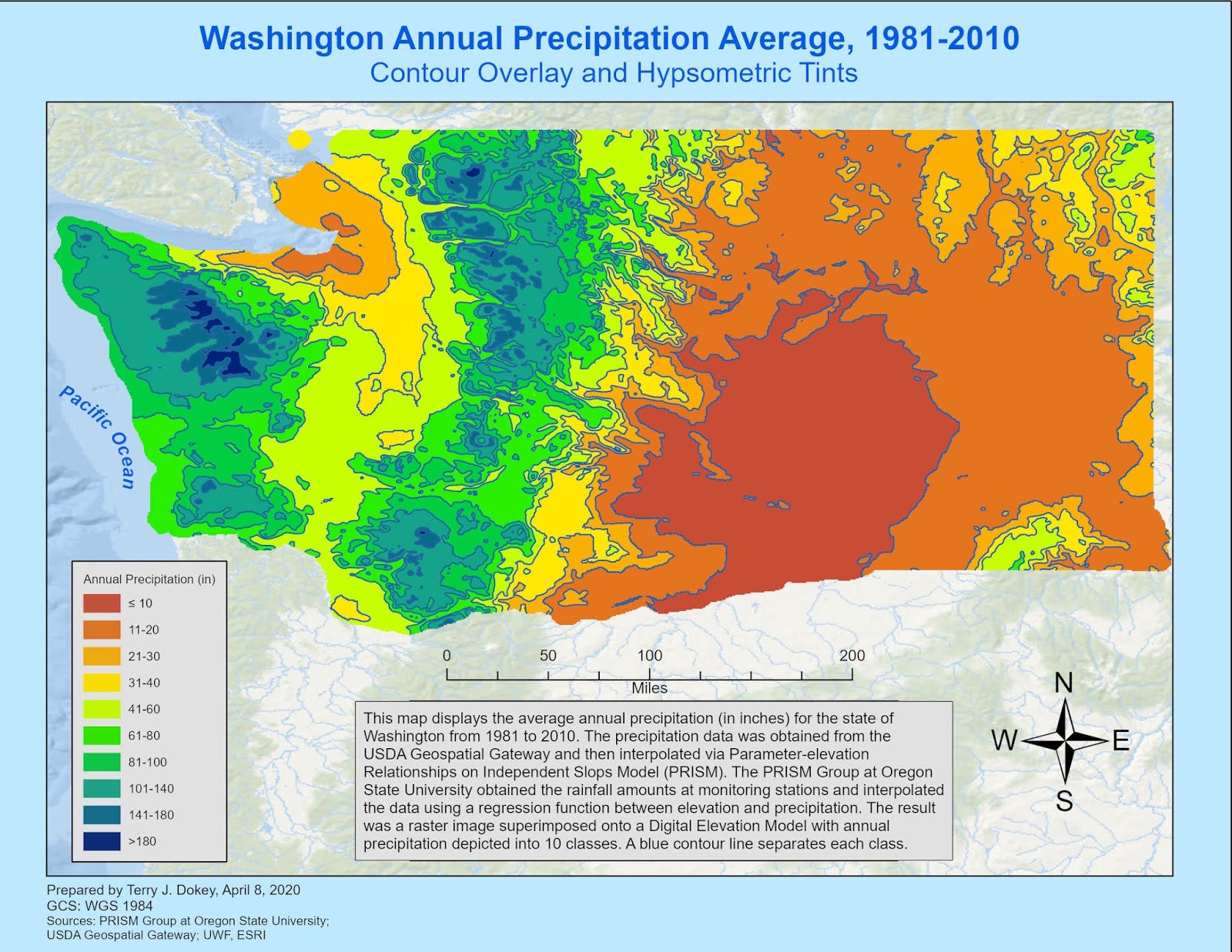Hypsometric Tints Isarithmic Map Depicting Annual Average Precipitation in WA

The final Hypsometric Tints map with contour overlay displays 10 classes of precipitation data that was collected from 1981 to 2010. All essential map elements are in place and I added a description box to further explain the map. All in all, it was a very straightforward lab assignment that provided more exposure and experience with raster images.