Module 6--Working with Geometries

Because of COVID, we were only required to do the last two modules. I completed M7 first, because it seemed easier.

In this module, I had to work with nested loops, search cursors, For Loops, and writing to text files for a system of rivers in Hawaii. The lab was very confusing and you definitely needed to use a pseudocode and to break up the lab into small parts. However, the exercise provided a base of knowledge from which to build upon.

Below are the results of the text file, which returned the Feature ID, Vertex ID, X and Y Coordinate, and the name of the feature:

Screenshot Showing OID, Vertex, X/Y Coordinates, and Name

Below is the pseudocode:

Start

               Import arcpy

               Import env from arcpy

               overwrite output = true

               workspace = “S:\GISProgramming\Module6\Data”

    new text file = “rivers_TJD.txt” (use the write function, “w”)

    fc = “rivers.shp”

               cursor = arcpy.da.SearchCursor(fc, [OID@, SHAPE@, NAME])

               use for loop through the cursor for each point

               vertex = 0

               vertex += 1

               f.write the results to the text file

               print results

               close text file

               delete row

               delete cursor

               print statement: The lab is complete

End

As always, take it one step at a time and look closely at indents, spaces, and other small issues to prevent syntax errors. Ensure you enable the overwrite function so you do not get the error code if you have to start another portion of the script again. Remember to think of the information you write as a table of columns and rows. Of course, the columns are the headers, OID, Vertex, X Coord, Y Coord, Name, etc. The rows are the actual features. Therefore, when you iterate over the loop, you are using {} to identify each column (e.g., {0} will be OID, {1} will be vertex, etc.).

Module 7--Rasters

Because of the shortened semester, we were allowed to choose between Module 6 and Module 7. I chose Module 7, which spoke about using rasters. In this module, I learned to import specific spatial analysis tools, ensure spatial analysis licensing was active, and create a raster map.

The module began with importing the typical modules and classes and setting the workspace environment. I then wrote a conditional statement (if/else) that would let me know if  the spatial analysis extension was available. After I checked out the SA extension, I reclassified the landcover map to only show forested land, input elevation, slope, and aspect functions, and then combined the rasters into one raster. Because these are not saved with the program, I added a save statement to ensure the raster was permanent. Because the raster ran, I knew the SA extension was good.

Raster image showing elevation, slope, and aspect for forest landcover

Module 5--Exploring and Manipulating Data

Well, I can guarantee that I am not quitting my day job. Though the lab started out easily, I got hung up on populating the dictionary. I probably spent 16 hours or more just one that one small step. After I finally figured out the issue, which was that by adding the update, get value statement for keys and values, and the key:value format statement within the for loop, everything printed out as required. I figured this out by commenting out lines of code and then adding new lines to see what happened. I eventually worked through the issues. Of course, viewing the student questions site on Canvas also assisted. Believe me, I contributed to the questions, but I also shared my solution.

The lab worked sequentially and built upon each step. Beginning with creating a new file geodatabase, I then assigned my feature classes to "fclist." I then copied these FCs to the new fGDB using a "for loop" (and also stripped out the .shp extension). Between each step, I learned how to add statements showing the date, time, and the amount of time the computer needed to complete the step. I also used "\n" to make sure lines were skipped for ease of viewing.

This screenshot shows the first several steps of the lab, to include the commentary: Create fGDB, copy Feature Classes, and creating a search cursor that returns county seats. The list of county seats is truncated to save space, but the code shows the information for all the county seats.

I then used a search cursor to sort out all the cities that were considered county seats in the feature column of the table. The only information I needed for this exercise was the name of the city, the feature, and the 2000 population.

Screenshot of the end of the county seat information. The dictionary is populated in the correct format {key:value}. Statements say how long it took, when the process finished, and the lab was complete.

Once I got the dictionary to print, the lab was complete. Though the lab was a challenge, I learned a lot.

A few words of advice:
--delete the row and cursor once you complete a loop.
--use \n so there is a line break.
--use print(arpy.GetMessage(count-1)) to get the date/time/process time for each line.
--don't forget the # symbol to add a comment.
--make sure ArcGIS Pro is not running at the same time as Spyder or you will likely get an error message.
--use the overwrite argument to reduce the amount of errors you receive saying that the fGDB exists (env.overwriteOutput=True).
--comment out lines of code (sometimes I put different numbers of # marks to keep myself straight) and try new lines. This way, you don't make a change and forget how to reverse it.

Module 4--Geoprocessing

During Module 4, I learned several tools to conduct geoprocessing functions using Python and Spyder. This was a much more enjoyable module because it allowed me to actually perform mapping functions. In other words, I saw the reason why we learn Python.

Some of the new tools I learned for Python:
--Model Builder, which actually built a model using a click/drag function and then having it perform the function. This is a much more visual method to use the tool.
--Buffering, to include dissolve.
--Clip, selects, erase tools.
--Add XY coordinates to a shapefile.
--Using the GetMessages() function to add commentary about the function performed.
--Make a toolbox.

Again, a few points to remember:
--Be very cautious of spelling (module, especially).
--Ensure capitalization is consistent with syntax.
--Consistency with quotation marks and contractions.
--Ensure URL of environment is accurate (spelling, slashes, etc.).
--Ensure comments section at top is complete (name, date, etc) using the # symbol.

Feedback of Hospital Script: Add XY Coordinates, Buffer,m Buffer Dissolve

The above screenshot displayed the results of the script written to add XY coordinates to the hospital shapefile, add a buffer, and then diffuse that buffer to a single feature. To complete this assignment, I broke the script into three parts, where I tested each script to ensure it worked properly before going to the next script. I also commented out commentary to explain what each step would perform. I used the GetMessages function to return the start time, date, etc.. I then added a print statement (separately) to return commentary on what the function performed.

All in all, this was an enjoyable module and a welcome change from the previous modules.

Module 3: Debugging

This module was much more straightforward than the prior. I am sure part of this is just the extra practice and increased understanding that goes with working through problems. I am glad that this module has been moved to earlier in the class so that we can find our problems in a systematic way.

During this module, we learned several ways to work through exceptions: Visual inspection of syntax, print statements, commenting out a line of code (or lines), and using the debugger tool in Spyder. I used all the tools throughout the exercise and assignment. Besides the visual inspection, I probably commented out several times to work through different versions of the script.

For Part 1, I just had to find two errors in the script. This was very easy, as this was just the warm up for the next two parts. When looking at syntax errors, the key is to consider indenting script properly and consistently, ensuring correct use of upper/lower case, symbols placement ("", :, etc.), and spelling.

Module 3, Part 1, Script 1

The above output was the result of correcting two script errors, which returned the feature classes in a geodatabase. A key to the exercise was ensuring that the scripts provided were in the correct location by verifying in ArcGIS Pro.

For Part 2, there were eight errors. These errors built onto the prior errors, but still contained many syntax errors. There was only one error that was a little difficult to find; however the debugger tool came in handy along with commenting out (using a #) and trying new lines of script. Once the script ran correctly, it printed out the names of the layers in the project's map.

Module 3, Part 2, Script 2

I was a little worried about Part 3 because it was the final step and I knew it would be the culmination of the entire module. For Part 3, we were expected to find an error, which was easy with the debugger tool. We were not supposed to fix the error, but use the try-except statement so that the script would execute with an easy to read statement and then continue to Part B. If correct, Part B would execute without error. The try-except statement was easy; however, it is imperative that you check your indenting so that those actions still remain within the script instead of outside. Below is the flowchart created to assist with this part.

Module 3, Part 3, Script 3

As you can see above, Part A ran, but returned an error statement that I had added to the code with my try-except statement. Once this executed, Part B ran and returned the names of the feature classes, data source, and spatial reference.

All my lessons learned are presented throughout this posting. A lot of this is just attention to detail. A big lesson learned for me was that everyone has errors and that many of the errors are simple spelling or punctuation mistakes. Look at those issues before deep-diving into the actual code. Additionally, the debugger tool is of great assistance.

Module 2: Python Fundamentals

For this week's exercise and assignment, there were numerous operations broken down into four steps. These steps included creating a string variable, creating a list, creating loops and iterating variables, and removing specific variables.

In Step 1, I created a string of my full name,  split the string to separate my individual names, and then used the index function to return a specific name. It is important to note that one uses 0 to return the first name and -1 to return the last portion of a string.

Step 2 required me to determine errors in a random dice game. This required me to first import the random module, which is the first line of code. I then looked at the script provided in the assignment to find two errors. A few things to note in errors: Ensure your quotation marks are not confused with contractions as it will confuse the program and return an error, make sure the case (upper/lower) is consistent, especially when naming a variable, and watch indention.

Step 3 caused me quite a bit of problems, as I overthought everything. In this scenario, I had to create a loop using a while statement and then append numbers to it until I reached 20 separate numbers. Again, this script required me to import the random module as the first step. One lesson I learned is that if you want to break the loop, the break must have the same indention as the loop. Otherwise, Python will return an error. I also learned that there are many different ways to arrive at a break statement.

For Step 4, I used the numbers generated in Step 3 (or I could have added this script to the script in Step 3). I then chose an integer as an unlucky number, used the while loop to remove the unlucky number, and then created a new list. This was fairly straightforward and of no issue. However, the next logical step in the future could be to remove the unlucky number and replace it so that there were still 20 numbers in the list.

Below are the results of my script, which has the return of each script. The explanations are written above, so I will not repeat them.

Script for Module 2. This shows the return items for each step in the assignment as explained above.

Flow Chart for Step 4.

GIS 5103--Programming--Module 1

After what seems like an eternity, classes have started again. This class will teach me how to write script using Python, which is the preferred scripting language for ArcGIS Pro. Though I was introduced to the Integrated Development and Learning Environment (IDLE), this class will use Spyder as the script editor. A word of caution is that if you use a virtual desktop, you must save the your products into the portal. If you were to complete the lab on your personal desktop and then dragged the finished product to the school's portal, there would be errors.

As part of the learning, we were introduced to The Zen of Python, which is a light-hearted set of guidelines for programmers. In a nutshell, the guidelines favor simplicity, utility, and practicality versus nested layers, complexity, etc. These guidelines also ensure Python can remain open source software and that others can add to its body of knowledge. Besides a few inside jokes in Zen, there is another: If you type in "import this" in Spyder, the Zen of Python will populate in Spyder.

The reading assignment also provided the steps to solve a problem for scripting. According to Agarawal et al (2010), I must first identify my inputs, determine the overall goals of the process, and then develop the steps to achieve those goals. Once I complete these steps, I can then write a pseudocode.  For this lab, I created a pseudocode for converting radians to degrees. The pseudocode must begin with Start and finish with End. All the interior lines are indented and completed in order with the variables placed prior to the actual operational function because the script runs in order from top to bottom and left to write just as we read. Once I created the pseudocode, I decided to convert this into Python script using Spyder, which yielded the correct computation. Prior to coding, I could have developed a flowchart, but I did not because it was a very simple computation.

For the lab deliverable requirement, I used Spyder and imported a .py file from the school portal (File>Open>*.py). Once I select the script and ran it (either using the run button or F5), eight folders (with three sub-folders each) populated into my share drive. This was important so that each student had the same folders. All data, scripts, and work will be placed in these folders in the future.

Screenshot of Lab 1 that Utilized Script to Produce 8 Folders in My Student Drive.

Though a little intimidating at first because I have never coded, the lab was very straightforward and there were very few pitfalls. My main pitfall was that I tended to overthink things. I have embedded many of my lessons learned throughout this post. One thing I did differently from the lab was that I went directly to Spyder from ArcGIS Pro instead of using the run option. To me, this was easier and saved a step. Another lesson is that when writing script, ensure that quotation marks are used following the command and be aware that a script must be saved prior to being run (the program will prompt you).

Module 6B--Flow Line Mapping

This was an optional exercise that utilized Adobe Illustrator in total to produce a map that shows immigration by continent and by percentage to U.S. states.

The assignment was great practice using AI and developing flow lines. Once all the objects were placed on the map, I chose to separate my continents and place them in an arc around the inset map of the United States (which already displayed the states as a choropleth map using five manually derived classes.

The biggest portion of the exercise was actually drawing the flow maps and modifying them to an appropriate shape. This was easy using the line tool in AI and then manipulating the anchor points. The challenge was determining the stroke of the line, which was proportional to the amount of immigrants to the United States. In order to determine the stroke width, I used an Excel spreadsheet that provided the immigration numbers for each region. I then determined the proportional weight by first determining the square root of each region's immigration numbers. From there, I used the following formula:

Width of Line Symbol = (Size of Largest Line I Want) * (SQRT of Region Immig/SQRT Max Value)

Though it seems difficult, it was very easy using excel. The only challenge to this was for converging lines, where you split the difference of the lines so that they converge to the proper width. The only reason this was difficult for me was because I tried to use lines that had transparency adjusted. This caused an overlap which I could not remove. If the lines are solid, this is not an issue. Another consideration is to make sure the lines do not overlap other lines or terrain and are presented appropriately. I chose to build my flow lines in a new layer and then placed this layer below the continents layer so that the flow lines originated from behind the continent and stopped short of the inset map. I then changed the colors of the lines to match the color of the continents. 

Once the essential map elements were built, I then modified the flow lines to show an inner glow, a drop shadow, and a bevel. The lesson here was that in the appearance tab, the bevel and extrude effect had to be above the inner glow and drop shadow so that the bevel was on the line and not the other effects. I then adjusted the bevel to make them look three dimensional and in perspective.

A word of caution, many of these effects (especially 3-D) use a lot of memory, which can slow processes or reduce the ability to add new effects. To finish the map, I used file-export to export the map to a .png file.

Flow Map depicting 2008 Immigration Numbers by Region and Percentage to each State.
Projection: Winkel Tripel

Module 6--Isarithmic Mapping

In this module, I learned about isarithmic mapping, which is a mapping method to present smooth, continuous phenomena such as precipitation, elevation, barometric pressure, etc. Besides the choropleth map, isarithmic maps are the most common, with the contour map being the most common isarithmic map.

In this lesson, I produced two maps. The data was obtained from the USDA Geospatial Gateway in raster format. The data had been prepared using Parameter-elevation Relationship on Independent Slopes Model (PRISM), which conducts a regression function between elevation and precipitation (in this case) for each digital elevation model (DEM) grid cell. Data obtained from monitoring stations are waiting based on their similarity to the grid cell. This has greatly improved data modeling and weather prediction.

The first map was a continuous tones isarithmic map that displayed average annual precipitation from 1981 to 2010 in Washington. Because it used continuous tones (stretching in ArcGIS Pro), it was much like a proportional symbols map in that the data was automatically converted into a color ramp which the program directed the stop points. Only the lower and higher numbers were displayed in the legend. I added the hillshade function to incorporate elevation into the map and adjusted its color ramp by editing each color stop by hue, transparency, and position on the ramp. Completion of the map was not required as it served more as a teaching tool and the origin of the hypsometric map.

Continuous Tones Map Isarithmic Map Depicting Annual Average Precipitation in WA

Once the continuous tones map was complete, I then produced a hypsometric tints map, displays contour lines between colors. This product started with copy/pasting the raster images from the continuous tones map. I then used the INT (Spatial Analyst) tool for the precipitation raster to convert the cell values to an integer. Using the precipitation color ramp, I classified the data into 10 classes. Because the class intervals were directed in the assignment, I used the manual function in the symbology pane.

I then created contours using the Contour List tool and aligned their intervals with the same intervals as the precipitation raster. The result was the contour lines appearing (in blue in the below map) between each color. The resulting final product is displayed below:

Hypsometric Tints Isarithmic Map Depicting Annual Average Precipitation in WA

The final Hypsometric Tints map with contour overlay displays 10 classes of precipitation data that was collected from 1981 to 2010. All essential map elements are in place and I added a description box to further explain the map. All in all, it was a very straightforward lab assignment that provided more exposure and experience with raster images.

Module 5--Choropleth Mapping

For this module, I produced a choropleth map that showed the population density of European countries along with wine consumption per capita. The task was to properly show both variables on the map using either proportional or graduated symbols. For extra points, I chose to use pictures of wine bottles in lieu of the default template (circles).

For the data display, I chose to use graduated symbols and the quantile data method with four classes. I did not need to normalize the data, because the data was already normalized in the attribute table (wine consumption per capita). To me, the quantile data method with four classes provided the best granularity to perceive and understand the differences in each variable. Additionally, I excluded four countries from the data set because they were outliers--high population density, tiny area, insignificant wine consumption. Additionally, the graduated symbols were easier to manipulate than proportional symbols. For proportional symbols, I had to set the lower limit and the sizes were manipulated automatically. For graduated symbols, I could manipulate the size for each class individually to ensure the viewer could perceive differences.

For the actual map, I used the Albers Equal Area Conic Projection because it was important to maintain the area throughout the map when comparing/analyzing data that has an areal perspective. I chose to use a purple color ramp to display population density because it reinforced and complemented the overall theme of the map--wine consumption. I also added an inset map to show the Balkans area, as this was too crowded on the main map to be usable.

Population Density and Wine Consumption (per capita) in Europe

I prepared most of the map in ArcGIS Pro. The biggest challenge was importing the wine bottles. In order to import the bottles, I found free, non-attribution clip arts that were in .svg form. I then imported the bottle and manipulated the size and other aspects to ensure that they would be added just like any other graduated symbol. In order to move the wine bottles, I converted the wine bottle symbols to graphics, which allowed me to move them. I did the same with the text to ensure there was no overlap and everything was sized appropriately.

For my base map, I used the Ocean base map in ArcGIS Pro. I then added bold italics names for each main body of water, though I altered the size based on the magnitude of the body of water. I also curved or bent my text to convey water flow.

Once all my essential map elements were complete, I then saved it as a .pdf because ArcGIS Pro no longer has the functionality to export to Adobe Illustrator. Once saved as a .pdf, I then opened a new project in AI from the .pdf file. I then touched up and added higher level graphics through AI: Moved wine bottles and names, added drop shadows to Atlantic Ocean, added inner halo in legend and other text boxes. I wanted to add an inner halo to the countries; however, this would cause issues with interpreting the population density. If this were just a regular map (not graduated), I would have added an inner halo.

The biggest issue for manipulating features in AI from a .pdf is that there are hundreds of components nested many times that you must manipulate. You must also control/click each component of the feature to ensure all are manipulated the same. For instance, I had a halo around the countries on the main map. In order to resize or move a country's name, I had to click on numerous components so that they were all changed in the same way.

 My advice to everyone is to be meticulous and systematic, especially when manipulating so many different features. I chose to pick a group of features and toggle between visible/not visible to locate it and then I manipulated as needed. Once I finished I went to the next feature in the right pane. Otherwise, it would be very frustrating to find the features by clicking on the map.

Overall, though very tedious, this was a fun exercise and I learned quite a bit. I can definitely tell that my competence and confidence have improved.

Module 4--Data Classification

In this module, I did a refresher on the four levels of measurement (nominal, ordinal, interval, and ratio) along with four common data classification methods to display on the map--equal interval, quantile, standard deviation, and natural break.

The exercise was very straightforward and built on skills previously learned. The task was to identify persons age 65 or over in the census tracts of Miami-Dade County. I then created two series of four maps looking at the data differently. The first series of maps displayed the four classification methods looking at the percentage of the population aged 65 or over in the census tracts. The second set of maps displayed the same methods but with the population normalized for square miles. As a reminder, choropleth maps should use normalized data.

The first set of maps is displayed below and shows the non-normalized percent of the population aged 65 or over:

Percentage of Persons Age 65+, Non-Normalized

As you can see, the data represents the percentage of the population for those census tracts presented in the four classification methods. In my opinion, the least useful is the equal interval method as it imposes artificial data breaks and generalizes the data too much. The quantile method is more effective, but also imposes artificial breaks. However, it provides much more detail, which is consistent with natural breaks and standard deviation. The standard deviation method assumes that the data is normally distributed. Because the data may not be normally distributed or may be skewed, this might not be the best method. Additionally, the data will be placed over six intervals based on +/- 3 std dev. Therefore, the majority of the data will be clustered around the mean and could be influenced by outliers. I personally like the natural breaks (Jenks) method as it utilizes an algorithm to establish intervals that minimize intra-class variance while maximizing inter-class variance. I believe that this provides the best representation of the data and takes into account natural clusters.

The second set of maps is displayed below and shows numbers (not percents) of persons aged 65 or over, normalized based on square miles:

Number of Persons Aged 65+, Normalized for Sq. Miles

The normalized data provides the number of persons aged 65 or over, normalized for square miles. I will not repeat my assessment of the data classifications, as they did not change. However, I acknowledge that choropleth maps should use normalized data. However, in this exercise, I do not believe it is necessary, though the purpose of the map would determine this. With this study, it considers how the people are spread across the area. Therefore, if a large amount of people are spread over a large area, their distribution could appear much smaller than a smaller amount of people compressed over a smaller census tract. Therefore, the data will favor the smaller areas and may not provide accurate results. For instance, if a commission wanted to allocate services to the elderly population, the number of people would be important, but not necessarily how they are in comparison to the area. To further explain my point, if a commission was setting up medical centers, a large area with a larger population may require more providers than a smaller area with a smaller population, even though the normalization will display a higher density in the smaller area.

Again, this was an enjoyable exercise and provides more considerations when designing maps.

Module 3—Cartographic Design in ArcGIS Pro

Module 3 was completed entirely in ArcGIS Pro, although I will likely import it to Adobe Illustrator just for practice. The lab was very straightforward and was a welcome refresher.

For this lab, I produced a map showing public schools in Ward 7 of Washington, D.C. I placed an inset map of Washington, D.C. with an extent indicator for Ward 7. The main map showed Washington, D.C. with Ward 7 in a lighter color. On this map, schools are displayed (in three hues and three sizes) by a school icon, roads are displayed as a line feature of varying weights and colors, and the Anacostia River is displayed by blue (lettering in italics to represent flow). Features not necessary for understanding were selectively excluded.

Ward 7 Public Schools: Cartographic Design using Gestalt Principles

One of the teaching points of this lab was to use Gestalt Principles in the map design:

--Visual Hierarchy— I arranged my map so that more important features stood out. Since schools were the focus of this map, I made the schools larger and brighter to draw attention. All other elements were relegated to a lower rank, to include roads. Interstates, State Highways, and major roads had lighter weights, respectively. Additionally, the roads were placed under the schools in the drawing order so that the schools were superimposed onto the roads if there were overlap. The remainder of the essential map elements were ranked in order of importance with the font and size of the item adjusted accordingly (example: Title was larger than subtitle; data sources was much smaller than subtitle). For areal features, I used lighter colors to draw attention. Therefore, Ward 7 was the lightest of the background colors.

--Contrast—I adjusted the weight of lines and color saturation just like in visual hierarchy. My schools were much brighter and I adjusted the school background to yellow in order to contrast with the background of the map. I made sure my background colors did not clash, but I ensured that areal features were lighter for Ward 7. For background information of lower importance (such as Ward 7 roads), the lines are barely visible so they do not compete with more important features.

--Figure-Ground—Just as in visual hierarchy and contrast, I adjusted colors and line weight to ensure important features stood out and looked closer to the viewer. The schools are different shades of red superimposed in a yellow circle to stand out from the grey background of Ward 7. Ward 7 is a lighter color to stand out from a darker shade of grey for the remainder of Washington, D.C.

--Balance—I utilized a sketch map as a tool to establish balance. Of course, Ward 7 was my main focus, so I centered the map inside a portrait orientation. I then used the open space to fill essential elements. I incorporated the inset map of the district in the upper left corner, which was balanced by the legend, cartographer information, north arrow, and data sources in the lower right corner. I placed the scale bar in the bottom center to balance the title and subtitle and I placed a list of schools (with numbers) in the upper right corner to balance the inset map and the legend group. I chose to place the inset map in the upper left corner because we read from left to right and this was more important than the name of the schools.

As previously stated, this exercise was very straightforward and completed in ArcGIS Pro. I input the data, which was obtained by UWF from District of Columbia Open Data. Once I produced the inset map of the district and the main map of Ward 7, I completed the map design process like previous maps. I ensured the scale was at an even ratio and placed a scale bar in miles with relatable and appropriate numbering. I chose background colors that were neutral, pleasing to the eye, and would add contrast to the schools and roads. In order to reduce the amount of information on the map, I selectively excluded features that were unnecessary for understanding—parks, minor roads, neighborhood clusters, etc.

Lab 2—Typography

Objectives:

--Produce a map in ArcGIS Pro, share to ArcGIS Online, input into Adobe Illustrator.

--Design a map and ensure all essential elements are in place.

--Label the map in accordance with typography guidelines.

--Utilize tools to symbolize and label features properly.

--Export the map to a picture file (.jpg).

For the Typography lab, I created a simple map of Marathon Key, Florida with an inset map of Florida. Once the maps were created and the coordinate system was set to Albers Conical Equal Area, I shared the map so that it would be visible in ArcGIS Online.

From there, I refined the map through Adobe Illustrator, which is a powerful tool to refine a map product. Though it is not very intuitive and can be rather daunting, it offers many more design features than ArcGIS Pro.

My main map is of Marathon Key, Florida at 1:100,000 scale. The inset map is the southern counties of Florida at 1:4,600,000 scale, as required in the instructions.

The inset map only displays the southern counties of Florida (in green to match the main map) with a red box showing the location of Marathon Key. In order to build a scale bar, I used simple division to convert the units of measure to a usable, even number. I then drew five alternating black and white boxes that were as wide as my number and assigned a representative distance. Ensure there is no stroke for the rectangles or the size will be larger than the scale represents. I added a border around the grouped rectangles by drawing a line the same size, increased its stroke, placed it behind the grouped bars, and then grouped the background and the bars.

For the main map, the colors of the land features match the colors of the inset map, but I adjusted the transparency to allow some terrain to show. To find the required features, I used Google Earth and plotted themed point feature symbols onto my map. Along with the themed symbols, I adjusted the size and color of the labels to correspond with the importance/significance of the feature (blue, italics for water; black for cities, brown for cultural, green for islands). For water, I either curved or waved the italics labels to represent water flow and adjusted the size of the label based on the relative size of the water feature.

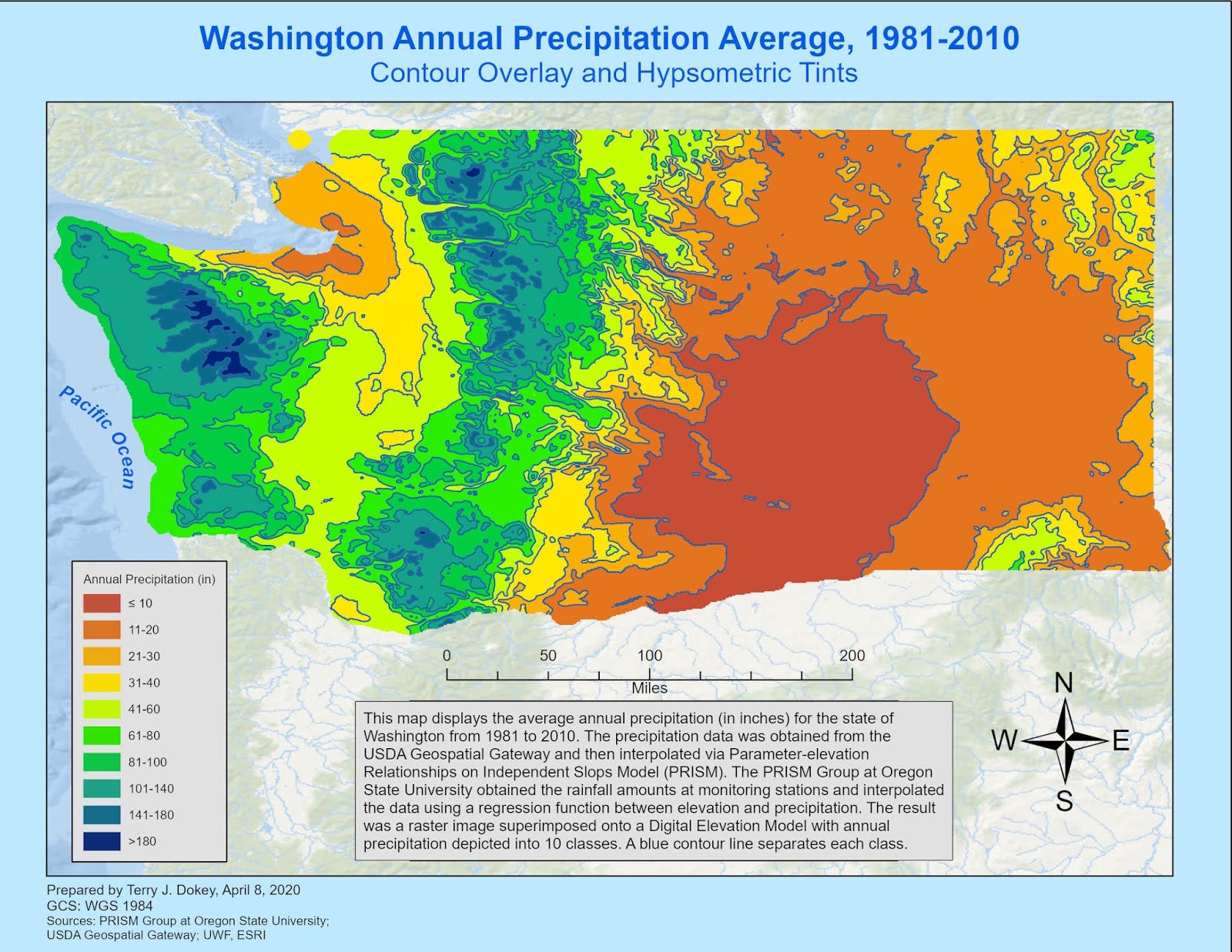
Marathon Key, Florida. 
Typography Lab, Module 2 in Albers Projection. Main map is at 1:100,000 and Inset is scaled at 1:4,600,000.

Because the map had many features close together, I used leader lines. I used the pen tool to draw the leader lines and ensured that they were the same stroke, generally the same angle, and did not touch the feature or label.

I then added the essential map elements:

--Border/Neatline—I added a rectangle and placed it at the bottom of the layout tab. I adjusted the stroke and color as needed.

--North Arrow—There is a symbol for this in the Symbols option, but I made sure it was not too large or obtrusive.

--Map Information—I used the Text tool (T) and added my name, date, and data sources in black with small font. I decided to add the GCS, too.

--Title and Subtitle—Used the text tool; used the largest font on the map and had it in bold/black to catch attention.

--Orientation—Landscape because of the size and shape of Marathon Key. If I had it in portrait, the map would have been very crowded and would not display required features.

--Legend—I used the rectangle tool and curved the corners. I then copy/pasted all the symbols that I used on the map and added labels. To improve the appearance, I used the alignment tools.

--Scale Bar—Was the most difficult portion for me because I overthought it. There are many videos that show how to make the scale bar with different systems, to include Adobe Photoshop. Though there is a method to create the scale bar, I was not able to manipulate the size or units while maintaining an accurate scale. I made Marathon Key’s scale bar as described above; however, I made sure there were smaller increments below zero.

Once I finished and refined the map, I exported it (check the "Use Artboard" option) to a jpeg file and then adjusted the resolution (high). Be sure to check the appearance of the photo so that nothing is distorted or misplaced.

In summary, I created the base map in ArcGIS Pro and then shared it to ArcGIS Online. I then imported the map to Adobe Illustrator and refined the map to be more presentable using the numerous tools and options in AI. I transformed the map (using the map board and compilation tab) into an Artboard, from which I modified Marathon Key to a finished product. In order to enhance my map, I used a drop shadow behind the islands, which provided depth. I also used themed point symbols as described above, and altered the color, size, and appearance of the labeling. I did not want to include too many customization, as this could turn into “map crap” and take away from the purpose. In the future, I will try inner shadows like one sees in atlases and large maps.

Though there was a steep learning curve to AI, I learned a lot. My recommendation is to follow any instructions closely, make sure the layer tab is organized, and to take your time. Walk away from the project for a bit if you get too frustrated. Also, leverage You Tube videos. There are plenty that show great tips and time-saving techniques.

Module 1--Importing ArcGIS Pro Maps to Adobe Illustrator

This assignment started out quite easily; however, I hit a few snags that I am trying to determine if it was my issue or an update to the software. Overall, it was a neat assignment and I am impressed how I can use ArcGIS Pro, transfer a web map to ArcGIS Online, and then export that map to Adobe Illustrator to actually design the overall map. I am not sure yet, but I think this might solve some of my best recommendations about usability and tools to design a map.

A few lessons learned, so far includes:
--I could not save my files directly from Adobe Illustrator, because it is on my personal laptop, whereas I use the GIS virtual desktop from UWF for all my GIS functions. I overcame this by saving those items to my desktop and then dragging them over to the share drive on the GIS portal. I am waiting to see if there is another method, so I don't continue to do this the hard way.
--I had serious issues finding some of the buttons for tools, especially the toggle lock tool to unlock editing to manipulate my extent. I never did find the tool and I am hoping to resolve this issue.

The results of the lab is the below map which was produced in ArcGIS Pro, exported to ArcGIS Online, and then exported to AI. I know I have a lot to learn, but I look forward to it.

Adobe Illustrator Map of Florida.

In the above map, the counties are outlined in black and colored in pink. Wetlands are colored in green and major cities and the capital are symbolized by dots. Since this was just a lab focused on learning the exporting procedures, I did not modify the symbols, as the cities are difficult to see and Tallahassee blends in with the other major cities symbols. Additionally, there are no essential map elements, as are generally required.

Module 1--Poorly Designed and Well Designed Maps

For the first module, I had to pick a map that well designed and a map that was poorly designed and critique it based on a template.

I had the opportunity to work in Washington, DC for almost five years. I will tell you that I was a little intimidated by the Metro until I road it the first time. People are justifiably proud of their Metro system (despite issues several years ago) and it serves the community well...it is indispensable.

DC Metro Map, Courtesy of WMATA, 2019.

As anyone can see, this is a very simple map that uses bold colors to show the Metro lines. The colors also correspond with the actual line names. Only basic information is added to the map to keep the viewer oriented. This includes the Potomac River in the middle, the borders of the DMV, and neighboring counties. The only element missing is the scale; however, this map is not drawn to scale (stated just below the north arrow). If it were drawn to scale, the map would be confusing, large, and not as intuitive. Besides, distance does not really matter. Time matters. Besides, most new riders and tourists track which station they need are heading to, the number of stations that have passed, and the number to go. To me, this is a very effective map.

On the other hand, I viewed the Easter Island map. At first blush, it appeared very good and I actually started my assignment choosing this map as a well designed map. As I went through the evaluation process, I changed my mind.

Easter Island, Courtesy of UWF.

There are a lot of issues with this map. Though it is attractive and centers on Easter Island, there are number of deficiencies:

--There is no title. I can assume Easter Island, even though the name of the island is in the water.

--The Moai represent Ahus and the Moai are represented by dots. This does not make sense, as the Moai symbols should represent Moai, which are ubiquitous to Easter Island.

--The Moai, ruins, and populated places are all symbolized by dots. It is difficult to tell which symbol represents which item, especially when dots are close together.

--The road symbols and the population symbols are not quantified.

--I am not sure what the names next to the Moai symbols represent--are these cities or the name of the Ahu?

--The scale bar has 5km,which is easy to relate to; however, the scale incorporates a little over 3 miles. I would have had two scales.

--Because the Easter Island scale has miles and kilometers, the inset scale should also have miles and the elevation scale (not labeled) should integrate feet.

Despite these issues, the map could be used for a middle school project to orient students. However, there is not enough information for a tourist map nor is there enough information or accuracy for a research project.

GIS 5007 Introduction

Well, I am beginning my third GIS course and my third course for this degree program. I look forward to learning about computer cartography, which will include Adobe Illustrator.

I joined this program because I am very interested in cartography. As a U.S. Army Infantryman, I was very reliant on maps and my ability to navigate. I developed a very keen interest in maps, so this was a natural fit for me. Additionally, the more I learned about GIS, the more I understood that its applicability is very wide and deep. It is not just about making maps, there are many other tools that use GIS as a base.

As I have stated before, I am very close to ending my 30+ years in the U.S. Army. All good things have to end and I have done my time...it's time for the younger folks to take over. Therefore, I wanted to obtain more technical skills, especially with regard to computers and information systems. Though I might regret it later, I am happy that I will learn some coding in future classes.

As part of this course, I had to create a story map on ArcGIS Online, much like the story map I created as part of my final project for GIS 5050. However, I did not use the Cascade version, but the newer version.

If you would like to look at my story map, it is at:

http://arcg.is/0uiOeO

or

https://storymaps.arcgis.com/stories/6f05cbc30b654d018578fd39e6edb8ab

I look forward to building my knowledge base throughout my studies.

URLs for Map Products

The cascade storymap and the commentary can be found at the following links:

Storymap:  http://arcg.is/1PPmK0

Commentary:  https://drive.google.com/file/d/1a5qgWWQ7dJly9i4synfSTqyrQxlcwxTG/view?usp=sharing

Summary of Final Project--Storymap

This was a very time-intensive project that brought all lessons learned in GIS 4043/5050. It was very rewarding and I continued the learning process throughout the design, research, analysis, and map production.

There are many lessons learned that I have captured in previous posts. As part of the project, I created a Cascade Storymap from ArcGIS Online. Though this had some excellent tools and attributes, I wish it had functionality a little closer to Power Point or other presentation tools. However, I do like that you can place an interactive map into the presentation.

Here are some of the tools I would recommend to be integrated:
--Ability to change font.
--Manipulation of each section to include picture placement, text location, etc.
--Ability to remove or re-position titles of slides.

The URL to my Cascade Map is:  http://arcg.is/1PPmK0

Below is my summary map that displays all criteria analyzed during this project. This summary map is also integrated into my Cascade Storymap as an immersive map.

Summary Map of Bobwhite-Manatee Transmission Project.
All features are added to this map and all symbology is consistent with
previous maps. This map is a "one-pager" that brings all criteria together and
presents the overall analysis.
Bottom line, the corridor meets all criteria and balances the need for additional
electrical power capacity with the impact on the environment and community.

Criteria 4--Length of Corridor

This portion of the project was quite easy. Again, I used imagery and previous feature classes in order to keep my colors and symbols consistent.

I created a new line feature and called it "PC Midline" and used the Project tool to make sure it had the same coordinate system as my base map.

To obtain the length, I used the Attribute Table and selected Statistics. This gave me the length, which I had to convert to miles. By my measure, the corridor was 24.52 miles.

As an optional task, I determined the overall project cost. To do this, I downloaded the MISO guide and estimated costs. This was a very easy to follow guide that took into account right of way costs, land preparation, foundation construction, tower components, etc. Though I am positive that I missed many aspects of the cost analysis, my estimate was approximately $21.1 million versus FPL's estimate of $20 million.

Imagery Map with PC Midline and Analysis of Length and Cost.
This map retains all features of previous maps and adds a purple midline
feature to the corridor. 

Criteria 3--Schools and Registered Daycare Centers

For Criteria 3, I had to define and quantify schools and registered daycare centers in proximity to the preferred corridor. I downloaded the U.S. Census Bureau's TIGER edge files for both counties and used imagery for my basemap. As with every map, I ensured that the GCS and projection were consistent.

I got a little over zealous on determining the schools and daycare centers. I prepared two separate Excel spreadsheets to input my data. Unfortunately, I input ALL schools and daycare centers in both counties from information on the school districts' webpages and a childcare center locator.

After I cleaned the spreadsheets, I save them in .csv format and then created my address locator. When I geocoded the schools, more than half were unmatched and would take an inordinate time to match them using Google Earth and school webpages. As a result, I located the zip codes that were impacted by the corridor and removed all schools (and later daycare centers) that were not in these zip codes. I then geocoded the result and matched any schools that were not matched. I did the same with the registered daycare centers.

Just as in the homes and parcels analysis, there were many schools and daycare centers that were new, had moved, or shut down. I had to use my best judgment when determining their status. In the end, only two private schools were within one mile of the corridor midline and no daycare centers were close. Therefore, no schools or daycare centers met the criteria to be impacted.

Schools and Registered Daycare Centers in Proximity of the Corridor.
The colors are consistent with previous maps. No schools or daycare centers
are impacted by the corridor.