Summary of Final Project--Storymap

This was a very time-intensive project that brought all lessons learned in GIS 4043/5050. It was very rewarding and I continued the learning process throughout the design, research, analysis, and map production.

There are many lessons learned that I have captured in previous posts. As part of the project, I created a Cascade Storymap from ArcGIS Online. Though this had some excellent tools and attributes, I wish it had functionality a little closer to Power Point or other presentation tools. However, I do like that you can place an interactive map into the presentation.

Here are some of the tools I would recommend to be integrated:
--Ability to change font.
--Manipulation of each section to include picture placement, text location, etc.
--Ability to remove or re-position titles of slides.

The URL to my Cascade Map is:  http://arcg.is/1PPmK0

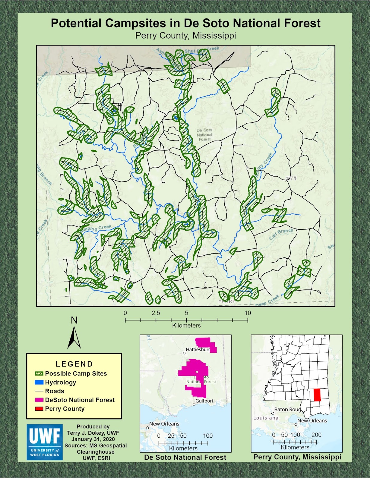
Below is my summary map that displays all criteria analyzed during this project. This summary map is also integrated into my Cascade Storymap as an immersive map.

Summary Map of Bobwhite-Manatee Transmission Project.
All features are added to this map and all symbology is consistent with
previous maps. This map is a "one-pager" that brings all criteria together and
presents the overall analysis.
Bottom line, the corridor meets all criteria and balances the need for additional
electrical power capacity with the impact on the environment and community.

Final Project Model

A requirement for the final project of the GIS 4043/5050 course is to construct a model that outlines a story map. The story map will assess the proposed route of the Bobwhite-Manatee Transmission Line through Sarasota and Manatee Counties, Florida. Though the line is already operational, it is a good assignment to bring together everything I have learned this semester.

To conduct the final project, I have to assess specific criteria: Impact on sensitive environmental areas and wetlands, impact on houses/parcels, schools, and registered day cares, and then determine the length of the proposed route and cost.

The model serves as a template much like an outline for writing a thesis. As shown below, the model begins with a problem statement, identifies data sets required, tentatively templates maps to be built, provide the GIS procedures to be used, and defines the result.

Though this model has been built, just like an outline, it is a living document and will evolve as the project progresses. However, it is a good tool to frame the project.

Final Project Model

Lab 6--Create a 3D Scene

Again, this portion of the lab built on the two previous products. By downloading a LiDAR layer from the National Map Viewer, I was able to create elevation and relief on the other layers.

To begin, I created a New Local Scene (Insert-New Map Dropdown) and added the LiDAR layer to the scene. In order to smooth the output, I filtered the image by selecting "Ground." I then searched for "LAS Dataset to Raster" in the geoprocessing pane in order to create a digital elevation model (DEM). When the DEM layer was selected, the image appeared to look like terrain features with different colors symbolizing different elevations. In contrast the previous incarnations were more pixelated and reflected off different surfaces.

Once the UWF buildings layer and roads layer were added to the resulting layer, they appeared to be "draped over" the terrain. For this project, I de-selected the DEM layer because I thought the World Elevation 3D/Terrain 3D layer looked better. Once this was complete, I added another layer for a map deliverable. Of course, the map had all essential elements. The only challenge was in rotating the 3D layer so that it was arrayed the way I wanted. There are many ways to do this; however, I went into the properties, and manipulated the degrees of rotation until I liked the result.
The resulting map is displayed below:

Map 3: 3D View of UWF Campus

The above map is the culmination of the entire lab. As stated, all essential map elements are present. The north arrow is arrayed to be the actual magnetic north of the raster layers. If I rotated the map, the north arrow would move in the appropriate direction. The original UWF roads are in red, the original UWF buildings are in light blue, Campus Lane (created feature) is purple, and Building 072 (created feature) is green. The scale bar is in feet because the overall map is in feet. I also added the map data which provides the author/date, sources, elevation ground surface method, and the RMSE and transformation degree.

Week 6--Editing

In the second part of Lab 6, I learned to create a new polygon feature and a new road feature. Though raster layers cannot be edited, new features can be added. This portion of the lab was straightforward and intuitive. To create both features, use the Edit tab, Features group, and click the create button. From there, create the feature desired. One caveat is to be cognizant of shadows on buildings as this could affect the overall size and shape of the building. Once the feature is saved, it appears in the attribute table, where the data can be edited (name, elevation, number, etc.).

The next portion of this lab required the creation of a Multiple Ring Buffer (MRB) to surround an eagle's next at 330 ft and 660 ft. Besides adding the picture to My Google Drive and adding the URL to the attribute table, I created the conservation easement using the MRB. This portion was very easy using the MRB Tool (Analysis tab, Tools, search). The only challenge I had was lining up the numbers in the MRB. I never did get it 100% accurate, but I got it close by using trial and error with the different offsets and array options. The resulting map is presented below:

Map 2: Bald Eagle Conservation Easement Using MRB

The above map was the result of the georeferencing in Part I and the editing of Part II. The main map shows UWF roads in red, Campus Lane (the new road feature created) in yellow, UWF buildings in lavender, and building 072 (the building feature created) in green. The MRB is in the lower right inset with the pink at 330ft and the light green at 660ft. In the main map, I placed a photo inset of the actual nest. To orient the viewer, the inset map of Florida displays Escambia County in red and points to the nest via a callout. The legend displays the different colors, the north arrow is oriented toward map north, and I have included sources, author/date, and the RMSE and transformation used. One lesson I learned through trial and error: You can de-select any feature in the expanded legend feature (content pane) by un-checking the box. This will prevent display of the RGB  boxes.

Week Six Lab--Georeferencing

Part I of this week's lab taught georeferencing. Two UWF (north and south) raster projections were added to the map. Once added, they appeared on "Null Island" off the west coast of Africa until the layers were georeferenced and "knew" their actual location. To move the image from Null Island, I clicked on the "Fit to Display" button. Once the image was located on top of the current layer, I added control points to align the image with the actual map. A few lessons: Spread out the control points, consider the effects of shadows on building geometry, zoom into the layers for accurate control point placement, and place the control point on the unreferenced layer first.

Review the overall Root Mean Square Error to determine how close the points were to the actual location. Remove control points (view the control point table) with high RMSEs to reduce overall RMSE. Then, determine the transformation to use. The higher the transformation level, the more control points (6 for 2d Order Polynomial; 10 for a 3d Order Polynomial) are needed and the more the raster bends.

Another very interesting portion of the lab demonstrated the techniques to place an unreferenced copy of a drawn map. Once I added the survey map (as imagery), I then georeferenced the map to the referenced imagery as before. This was much more difficult because the map was much older, had limited information, and skewed excessively if control points were placed too close (next to each other versus opposite sides of the image).

Heritage Hall Georeferenced

The above image is the result of georeferencing a parcel survey and then placing it on a UWF Campus image. The control points are shown in red (parcel survey) and green (image) and the overall RMSE was 6.770932. The most efficient way to place control points was to use the edges of parking lots and the points of medians, since no buildings were drawn on the parcel survey. Again, place control points on opposite ends of the image (much like you tighten lug nuts on a tire) to reduce distortion. 

Geocoding

This week's lab taught me quite a bit. Though I am still weening myself from Power Point habits, I was excited to learn some Excel techniques. I wish I had known about these time-saving tools several years ago.

The lab started by converting latitude/longitude (DMS format) into decimal format via Excel. Once I set up my headings in the spreadsheet, I used the extract function to remove specific characters (by Left or Mid, place number, and number of characters) from one cell to another. As with all Excel functions, I was then able to drag the formula down the column, saving time. Once the D-M-S (use a comma for degrees) were extracted, I then converted the numbers into X and Y coordinates (decimal form). Once I added the data to a new project, the eagle nest locations were displayed.

Eagle Nests. Hybrid imagery of Santa Clara County, FL. Green point features are eagle's nests obtained by converting lat/long to X/Y decimal coordinates. The XY Point Data was then added to the layer group to display the locations.

The second part of the lab taught geocoding. To accomplish this, I downloaded census data (TIGER) and addresses from Brevard County Schools. Once the data was placed into Excel, I converted the addresses for input into the address locator function. Using Excel extraction functions and offset functions, I stripped specific data from a cell and moved it to another. Following each operation, I copy/pasted the values only into another spreadsheet (tab at bottom). To remove excess cells (many of the input data took up multiple cells), I used the filter function, which allowed me to select/de-select data within columns and then perform a function (such as delete).

Brevard County Schools. This is a hybrid imagery map of Brevard County, Florida. In this map, yellow outlines are roads and boundaries. The purple school point symbols are Brevard County schools. The data was obtained by downloading standard mailing addresses and transforming the data into a usable format to be geocoded in the address locator. After matching and re-matching the output, the schools were displayed with the school house symbol.

When the addresses were formatted properly (saved in an .xls and .csv format), shapefiles were added (roads and county boundaries) and the projection was changed. I imported the .csv table and created an address locator, which allowed me to geocode. By geocoding, each address was matched to a specific map location. Those unmatched schools were rematched using Google Earth and sometimes visiting the school website. From this analysis, I located the school location, I chose its site on my map. For ease of viewing, I changed my school icons and saved my data.

The link to the above web map is http://arcg.is/ai1vP

All in all, it was a fun lab. I always enjoy learning, especially when I can leverage the new knowledge into future projects (such as the new Excel tools I learned).

Lab 4--Vector Analysis Part I and II

This was an interesting and fun lab. It is important to understand the difference between a feature class and shapefile. A feature class resides inside a geospatial database. Though the feature class can contain shapefiles, all elements of a shapefile must have the same geometry (point, line, or area).

An attribute table is a powerful tool that must be learned. An attribute or location query is the starting point to select or exclude specific criteria and modify the feature class to portray the desired results. As an example, a realtor might develop a query to select all houses 500 meters beyond a flood zone (or remove all houses within 500 meters), within 5 miles of a school, and within 10 miles of a fire station. The resulting output produces prospective houses meeting the buyer's criteria. Variations of this function include intersecting features (feature is partially in the area), joining tables (includes features of both tables), and producing compound (multi-ring) or variable buffers (different features have different distances from an area). An alternative to the aforementioned processes is to perform a union.

To produce my final product, I imported database files from the Mississippi Geospatial Clearinghouse. With this data, I could isolate MS counties and select the De Soto National Forest (near Hattiesburg, MS). Not only did I import new feature classes, but I also built my layers, produced buffers, intersections, joins, and exclusions. The resulting map depicts potential campsites in the forest, with selections depicting areas outside the buffer of drain basins, rivers, lakes, sensitive land areas, etc. 

I designed the overall map  to appeal to outdoor-oriented persons. I added two inset maps to orient the viewer to the location of the National Forest and Perry County. All essential elements of the map were input (north seeking arrow, name/date, credits, scale, neat line, etc.) to ensure the map was easy to read and understand, uncluttered, and accurate. 

Specific Map Elements:
--Legend: Displays all features of the map and inset maps with standardized colors.
--Colors:
   -Hatched green--potential camp sites (intersection of water/road buffer join and sensitive areas).
   -Blue--all hydrology.
   -Black lines--Roads
   -Red--Perry County
   -Pink--De Soto National Forest
--Map Scale: Specific for each map based on most effective display.
--Scale Bar: Even number of kilometers (projection based on meters) and suitable for the size of the area.
--North Area: Map north. I did not use true north because I would have had to have a different arrow for each map or the maps may have been rotated in odd directions. Map north is easier to view and understand.
--Titles: Explain the purpose of the overall map and the location.

Though this lab continues to build proficiency, there are some lessons:
--Always ensure your selections are cleared before executing another selection-type process.
--Make sure your drawing order is arranged properly so you can modify features on a particular layer.
--Be prepared to change your database format in the event that it is wrong or outdated (File>Options or Metadata>Update, respectively).
--When modifying a feature class, make a copy (and rename it) so its original content can be added to another layer.
--Once you begin making your map, do not move your database files or rename them. Your map will be affected negatively. Be careful on what files you delete as some may be more necessary than you thought.

Lab 4--Vector Analysis Lab Showing Potential Campsites
within the De Soto National Forest, Hattiesburg, MS.

Update to this Lab: I neglected to set parameters for different classes of campgrounds. Therefore, if you use this as an example, be advised, that I missed this point in the instructions. Just make sure you set up some parameters to delineate different types/qualities of campgrounds based on the terrain.

Projections

In this lab, I learned to download data (from FGDL) and input it into a project. We then explored projections and learned that ArcGIS Pro requires data sets to be in the same projection (on the fly reprojecting) to be displayed together and have full functionality for analysis.

To demonstrate how different projections alter the orientation, size, compression, etc. of map features, I compared four Florida counties. By transforming the county data set to Albers, UTM, and State Plane, I produced three maps with an associated data comparison of area.

I then worked with raster projections and learned to input my chosen coordinate system. This will ensure the JPEG World File (.jgw) will have the correct coordinate system, resulting in a correct location display. I am very comfortable with UTM, because I am in the military and work extensively with MGRS, which is based on UTM.

Comparison of County Area Outputs Using the Albers, UTM, and the State Plane North Projections

Produced by Terry J. Dokey, January 22, 2020

Google Earth

After collecting the data in Collector, the lab required me to share the data as a Google Earth file and an ESRI map package. I created two .kml files (.kmz if in zip format)--one from ArcGIS Pro and one from ArcGIS Online. This was very easy, but the files were much different in size and in the way the data was portrayed.

I imported both .kml files to Google Earth Pro (online). I was unable to display the files simultaneously, but I could toggle between both files. As with all Google Earth applications, the output was beautiful and I could pin the data for others to see.

I also created a map package to share a map with someone not connected to the network. This operation was very easy, to include the synchronization between ArcGIS Pro and ArcGIS Online. This is a very powerful tool in the event that someone does not have access to these programs, which are very expensive.

All in all, I really enjoyed this lab and look forward to building my knowledge base further.

ArcGIS Collector and Sharing Maps

Lab 3 was quite fun and creative. I was introduced to ArcGIS Online, which synchronized with ArcGIS Pro at my work station. Additionally, I operated ArcGIS Collector, an intuitive, powerful tool, especially for emergency management personnel. The assignment required me to pinpoint five public safety objects and plot them on a map via Collector (real time or offline). I chose fire hydrants because of their importance and effect on rental insurance premiums.

In ArcGIS Pro, I created domains (parameters and descriptions of the feature class) for the fire hydrants. I portrayed the fire hydrants' condition using a Red-Amber-Green format (with a qualitative definition). The steps were straightforward and intuitive, and the concepts built upon the previous lab assignments.

Once the feature class was complete, populated to my map, and scale and extent were updated, I shared my map as a "Web Layer" with the UWF persons. This option is unavailable unless you are signed into ArcGIS Pro. Once I configured the feature layer and analyzed for errors, I published the map, which populated onto ArcGIS Online (must sign in).

I adjusted the feature layer, I added it to my web map and shared with UWF.  I easily downloaded ArcGIS Collector to my Android phone and added locations and pictures to my map, taking less than 30 seconds per location. The map updated in real time on my phone. When I opened ArcGIS Online, my points were also updated and could be opened on ArcGIS Pro. I was very impressed that all my points, descriptions, and photos were either plotted on my map or available by clicking the location.

My story map is located at  http://arcg.is/1SmXXX if you have access to ArcGIS Online, UWF Group.

University of West Florida Main Campus
Produced  by: Terry J. Dokey, 1/17/2020

This is my Lab 2 Assignment, Cartography.  This map is designed for visitors who wish to know a macro-scale version of the location of the University of West Florida. The map is not intended for navigation, as I have shaded the different areas and only highlighted (in color) important points.

In the upper right hand corner, I have an insert that shows the state of Florida's counties in grey and Escambia County, the location of UWF, in pink.

The main portion of the map has Escambia County in transparent pink and the surrounding counties in transparent green.  The major rivers are in blue, the main interstates are in red, only the two largest neighboring cities. Because UWF's location is the purpose of the map, it is symbolized with a star.

To ensure the viewers could orient and understand the map, I included a north seeking arrow (upper right), a scale in both the insert and the lower portion of the main map, and a legend (lower right).  I also included cartographer and bibliographic references to ensure credibility, attribution/credit, and ensure reproduction.  Finally, I added the UWF symbol to dress things up and further demonstrate the purpose of the map.

I chose all the colors to work with the best interest of the viewer. Everything I have learned so far demonstrates that the map is a contract between the cartographer and viewer. Therefore, all elements should be approached with the viewer and purpose in mind.

Lab 2--Cartography

Today I finished Lab 2, Cartography, which taught me how to produce a map (with an insert) plus add essential elements of map information, which includes the legend, north arrow, bibliography, date, cartographer's name, etc.  This lab was truly fun and there was not much frustration to it. By doing and re-doing the labs, I have learned that steps that caused frustration are no longer frustrating me.

Along with another student, I served as the discussion leader for the class.  This entailed me completing the lab, offering tips and techniques, and then answering questions from the students. This is a very good technique for many reasons:  It forced me to learn more quickly; as a graduate student, it allowed me to serve at a higher level (plus higher expectations) than the undergraduate students; it provided more time for the professor to tackle more difficult problems; facilitated better communication and increased the likelihood that a student would ask for assistance because the discussion leaders are students, too, and are less "threatening" than approaching the professor.  All in all, this was a good week and I truly look forward to the next lab.

Becoming Fun

As I practice more with ArcGIS Pro, it is becoming much easier and I am not making the same mistakes.  The biggest challenge for me has been the terminology for the different frames, views, etc.  However, it is becoming much more fun as the processes are becoming more automatic and I am able to be more creative. I am looking forward to gaining proficiency and integrating this into future jobs.

Continued Improvements

Today I attempted to improve my blog.  The only thing I was really able to accomplish was adjusting fonts in the design tab and converting a few pictures into actual hot buttons.  I haven't quite cracked how to make the post better using a free system.  Maybe one day...

Lab Assignment 1

Today, I completed the first lab assignment.  It was a little bit of a challenge for me, but I mitigated quite a bit of the challenge by having two monitors.  I definitely recommend that you have about a 24 inch monitor in addition to your laptop monitor. It made things quite a bit easier and reduced the amount of clicking and minimizing.  The instructions for the lab were very easy to follow, but I second-guessed myself for the file path because the abbreviated example did not contain the same data.  I have also learned that I reduce my frustration by first downloading the process summary and printing the instructions and then logging onto Google Drive and opening the GIS application.  This way, I can have all the information I need without moving between the virtual desktop and my own desktop.  All in all, it was a fun assignment, but I think I will practice a little more so that I can seamlessly navigate between folders before the labs become more difficult. As for the map itself, I just followed the instructions as written to include the symbology choice (Circle 1).  I chose green for my color ramp because I wanted it to transition from lighter to darker and I did not want to use blue because I felt it would confuse the viewer because the oceans are blue. I then saved it to the S drive and the Google Drive.

Terry's Lab 1 Deliverable--World Countries (Topographic)

Coding Attempts

Fellow GIS 5050 students,  I am still working with this and trying to learn codes to make my blog more attractive. Bear with me, please...

Label Gadget Test

Just doing a test to make sure the label gadget works. As I stated, this is all new to me.

First Blog Post Ever!

Well, this has been a learning experience figuring out how to blog.  Should be an interesting journey, but I am looking forward to it.